Advanced Monitoring Strategy

• the requirement on the number of switches of different monitoring wavelengths;
• limitations for a signal swing;
• amplitude of a signal variation between adjacent extrema values;
• deviations between TL and adjacent signal extremum value.

The strategy is available at:

Results –> Monitor –> Strategy button –> Strategy 4

Amplitude of the monitoring signal is the difference between its maximum and minimum:

\[ A=V_\max-V_\min \]

Initial and final signal swings (\(S_{in}\) and \(S_{max}\) ) are defined for each coating layer and calculated as follows:

\[ S_{in}= \frac{V_\max-V_{in}}{A}\cdot 100\%, \]if the first extremum is maximum;

\[ S_{in}= \frac{V_{in}-V_\min}{A}\cdot 100\%, \]otherwise.

\[ S_{fin}= \frac{V_\max-V_{fin}}{A}\cdot 100\%, \]if the last extremum is maximum;

\[ S_{fin}= \frac{V_{fin}-V_\min}{A}\cdot 100\%, \]otherwise, where \(V_{in}\) is the signal level at the start of the layer deposition, \(V_{fin}\) is the termination level.

In the case of a thin layer, having no extrema of the monitoring signal inside,  OptiLayer considers continuously increasing thickness of the monitored layer above its nominal thickness until the next two extrema appears on the monitoring curve. These two virtual extrema are considered as the first and the last one in the conditions above.

Evidently, swing values close to 0% and 100% mean that signal is close to extremum values. Initial swing for the first layer is always equal to zero.

Another important parameter is the difference between the termination level \(V_{fin}\) and the next signal extremum \(E_{next}\):

\[\Delta=|V_{fin}-E_{next}|\]

OptiLayer chooses monitoring wavelengths in order to satisfy the following five monitoring conditions:

• The number of monitoring wavelength changes does not exceed five. Actual number of different monitoring wavelength changes, allowed spectral range for their choice, and the wavelength grid step for this choice are specified by an optical coating engineer;
• \(a_1\le S_{in}\le a_2\), i.e. initial swing should not be too small and too high (the first layer with should be excluded);
• \(b_1\le S_{fin}\le b_2\), i.e. final swing should not be too small and too high;
• \(A\ge\epsilon\), i.e. signal amplitude should not be too small;
• \(\Delta\ge \delta\), i.e. the distance between termination level and the next virtual extremum should not be too small.

The values \(a_1, a_2, b_1, b_2, \epsilon, \delta\) are the parameters of the algorithm. The conditions are connected with the requirement that termination levels should be located at signal slopes with enough steepness. For example, reasonable values of these parameters are \(a_1=a_2=15\%,\) \(b_1=b_2=85\%\), \(\epsilon=4\%\), \(\delta=4\%\).

Generally, it may be not possible to find a sequence of wavelengths so that all conditions are satisfied simultaneously for all coating layers. Our algorithm chooses monitoring wavelength(s) so that the conditions are satisfied as close as possible.

It may happen that some conditions are more important than the others. For such cases, condition weights are introduced. The weights allow you to adjust relative importance of different conditions.

Bad Monitoring control allows you to visualize layers having monitoring signal with bad quality for reliable monitoring purposes.

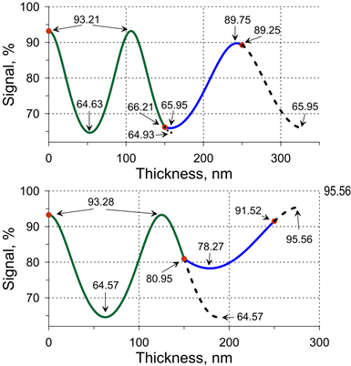
Fig. 1.

Illustrating example: a model coating consisting of two layers on a Suprasil substrate; layer refractive indices equal to 2.35 and 1.45, layer physical thicknesses equal to 150 nm and 100 nm.

The corresponding signal for the case when monitoring wavelength is 500 nm is shown in Fig. 1 (upper panel). The corresponding parameters for Layer 1 are:

\[ A=93.21\%-64.63\%=28.58\%>\epsilon=4\%,\]

\[ S_{in}=0, \; \mbox{(excluded)}, \]

\[ S_{fin}=\frac{93.21\%-66.21\%}{28.58\%}\cdot 100\%=94.47\%>a_2=85\%,\]

\[\Delta=66.21\%-64.63\%=1.58\%<\delta=4\%.\]

The parameters for Layer 2 are:

\[ A=89.75\%-65.95\%=23.8\%>\epsilon=4\%,\]

\[ S_{in}=\frac{66.23\%-65.95\%}{23.8\%}\cdot 100\%=1.2\%<a_1=15\%, \]

\[ S_{fin}=\frac{89.75\%-89.25\%}{23.8\%}\cdot 100\%=2.1\%<b_1=15\%,\]

\[\Delta=89.25\%-65.95\%=23.3\%>\delta=4\%.\]

It is seen that some conditions are are satisfied, and others are violated; termination levels are very close to signal extrema.

Application of our algorithm gives the monitoring wavelength of 588 nm. The corresponding monitoring signal is shown in Fig. 1 (lower pane). The parameters are now for Layer 1 as follows:

\[ A=93.28\%-64.57\%=28.71\%>\epsilon=4\%,\]

\[ S_{in}=0, \; \mbox{(excluded)}, \]

\[ b_1\le S_{fin}=\frac{93.28\%-80.95\%}{28.71\%}\cdot 100\%=42.9\%\le b_2=85\%,\]

\[\Delta=80.95\%-64.57\%=16.38\%>\delta=4\%;\]

and for Layer 2:

\[ A=95.56\%-78.27\%=17.29\%>\epsilon=4\%,\]

\[ a_1=15\%\le S_{in}=\frac{80.95\%-78.27\%}{17.29\%}\cdot 100\%=15.5\%\le a_2=85\%, \]

\[ b_1=15\%\le S_{fin}=\frac{91.52\%-78.27\%}{17.29\%}\cdot 100\%=76.6\%\le b_2=85\%,\]

\[\Delta=95.56\%-91.52\%=4.04\%>\delta=4\%.\]

All conditions for both layers are satisfied.

Example 2. 8-layer AR coating works in the spectral range from 650 nm to 750 nm, and in the angular range from 0 to 70 degrees; light is non-polarized;   substrate is Suprasil, layer materials are Nb₂O₅ and SiO₂. Reflectance in the working spectral and angular ranges does not exceed 9.2 %.

A monitoring wavelength the wavelength of 700 nm is located in the middle of the antireflection spectral range.The corresponding signal is depicted in Fig. 2 (upper panel).

The advanced algorithm proposes the wavelength of 621 nm (corresponding monitoring signal is plotted in the lower panel of Fig. 2.

Fig. 2.

In order to compare the monitoring wavelengths of 700 nm and 621 nm from the practical point of view we perform a series of computational manufacturing experiments in order to estimate production yields.

Production yields for the wavelengths of 700 nm and 621 nm are estimated as 0.2% and 98.6%, respectively. See the details in Monochromatic Monitoring Simulation.