|
Measurement data obtained in-situ can be easily imported and loaded to OptiLayer using Multi-Scan Measurements Manager available in OptiRE through Data –> Multi-scan measurements. In the lower part of the window Measurements database is displayed. The upper part displays layers of the design currently loaded to memory (see below). Load button loads selected measurement data file to the position selected by an arrow in the design. This position correspond to measurements performed after the deposition of the selected layer. Alternatively you may use Layer column in order to assign a layer to a measurement data file. Unload button removes measurement data from the selected position in the upper part of the window. MultiLoad… button invokes a special three-step dialog allowing to perform massive and automated multi-scan measurement assignments. Unload button allows you to unload selected measurement file from memory. It is also possible to unload all measurements from memory at once using popup menu invoked after clicking a small arrow at the right part of the button. Reload button allows you to load measurement file from the database again discarding all possible in-memory modifications, for example, results of measurements preprocessing. |
|
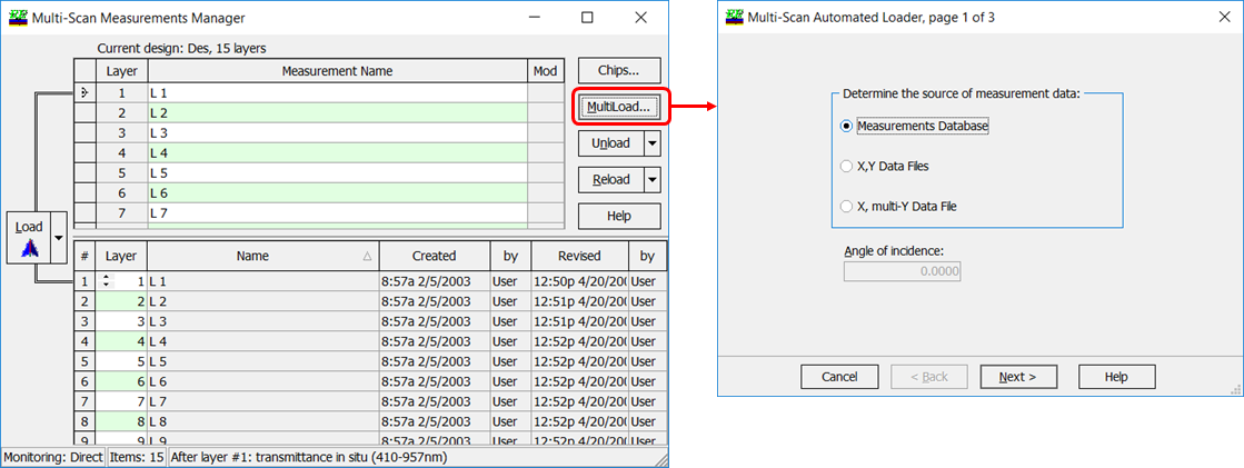
Example: loading multi-scan data that is already in the OptiLayer database. |
|
| Using Scan Discrepancies Option available through
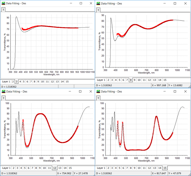
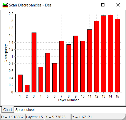
View –> Scan Discrepancies, you can plot discrepancies between theoretical (or model) spectral characteristic and corresponding measurement scan. Example: Comparison theoretical and measurement transmittance data related to a 15-layer beamsplitter. The data corresponding to the 3rd, 8th, 12th, and 15th recorded scans are shown below. The scan discrepancies are represented on the right panel.
|
Discrepancies window represent partial discrepancies \(D_j, j=1,…,m\), \(m\) is the number of design layers for the multi-scan measurement mode:
\[ D_j=\frac 1L\sum\limits_{i=1}^L \left(T(d_1,…,d_j;\lambda_i)-\hat{T}(\lambda_i)\right)^2, \] where \(\lambda_1,…,\lambda_L\) are measurement spectral points, \(\hat{T}(\lambda_i)\) are measurement values. The scan discrepancies are represented as a diagram (see below) or in a numerical form in Spreadsheet tab.
|
| Efficient numerical algorithms provided by OptiRE enable performing reliable reverse engineering of multilayer coatings. We demonstrated reliability of the reverse engineering results obtained on the basis of multiscan measurements in our publications.
Recent version of OptiLayer allows you to analyze BBM movies. Example: a special 15-th layer quarter wave mirrors was produced and two errors (+5% and -7%) in layers 3 and 12, respectively, were imposed. Layer materials – Ta2O5, SiO2; Glass substrate, central wavelength – 600 nm. Deposition technique – magnetron sputtering. Thickness control – well-calibrated time-monitoring. In the course of the deposition process, transmittance data scan were recorded insitu after each layer. The experimental data are compared with the theoretical ones below (left panel). A model with random errors was applied, i.e. the diecrepancy function \(DF\) was minimized with respect to relative errors in layers thicknesses \(\delta_1,…,\delta_{15}\): \[ DF^2=\frac 1M\frac 1L\sum\limits_{i=1}^M\sum\limits_{j=1}^L\left(T(d_1(1+\delta_1),…,d_m(1+\delta_m))-\hat{T}(\lambda_j)\right)^2 \] |
|

Initial fitting of in situ measurements recorded after each layer by theoretical transmittance of 15-layer quarter wave mirror. |
Achieved fitting of in situ measurements recorded after each layer by model transmittance of 15-layer quarter wave mirror. |
|
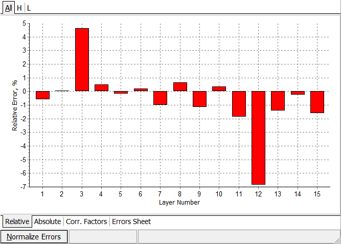
Estimated relative errors in layer thicknesses. Two errors in layers number 3 and 12 are reproduced with high accuracy. |
|
Evolutionary Reverse Engineering Algorithm |
|
| New evolutionary post-production characterization algorithm significantly improves the search for the best fit in the case of multi-scan data. The new option is available in OptiRE through:
Solve –> Random Errors Solve –> Quasi-Random Errors Solve –> Quasi-Random Inhomogeneities Solve –> Random Errors (scientific mode) Solve –> Quasi-Random Errors (scientific mode) |
|
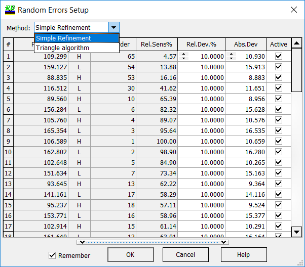
| In comparison with the previous versions, there is a choice between two algorithms in “Method” field: Simple Refinement and Triangular algorithm. In the case of “Simple Refinement”, discrepancy function \(DF\) is minimized with respect to all “Active” layer thicknesses:
\[ DF^2=\frac{1}{m}\sum\limits_{k=1}^m\frac 1L\sum\limits_{j=1}^L\left[\frac{T(d_1,…,d_m;\lambda_j)-\hat{T}^{(k)}(\lambda_j)}{\Delta T_j}\right]^2, \] where \(m\) is the number of design layers, \(\{\lambda_j\}, \; j=1,…,L\) is the wavelength grid, \(\hat{T}^{(k)}(\lambda_j)\) transmittance scan recorded after the deposition of \(k-\)th layer, \(\Delta T_j\) are measurement tolerances. |
 |
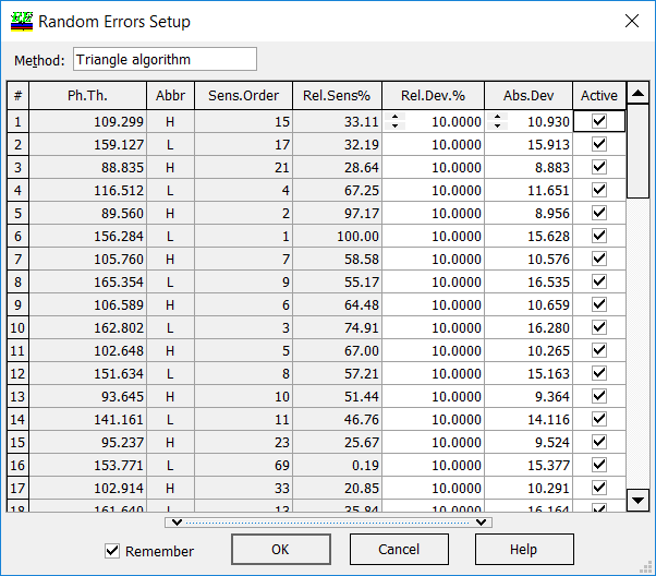 |
In the case of “Triangular algorithm”, partial discrepancy functions \(DF(i)\) are minimized with respect to all “Active” layer thicknesses among \(d_1,…,d_i\):
\[ DF^2(i)=\frac{1}{i}\sum\limits_{k=1}^i\frac 1L\sum\limits_{j=1}^L\left[\frac{T(d_1,…,d_i;\lambda_j)-\hat{T}^{(k)}(\lambda_j)}{\Delta T_j}\right]^2,\] where \(m\) is the number of design layers, \(\{\lambda_j\}, \; j=1,…,L\) is the wavelength grid, \(\hat{T}^{(k)}(\lambda_j)\) transmittance scan recorded after the deposition of \(k-\)th layer, \(\Delta T_j\) are measurement tolerances. Important: At each \(i-\)step, starting approximations of actual layer thicknesses are taken from the result of the \((i-1)-\)step. This reduces the instability in determination of actual layer thicknesses significantly.
|
OptiLayer provides user-friendly interface and a variety of examples allowing even a beginner to effectively start to design and characterize optical coatings. Read more…
Comprehensive manual in PDF format and e-mail support help you at each step of your work with OptiLayer.
If you are already an experienced user, OptiLayer gives your almost unlimited opportunities in solving all problems arising in design-production chain. Visit our publications page.
Look our video examples at YouTube
OptiLayer videos are available here:
Overview of Design/Analysis options of OptiLayer and overview of Characterization/Reverse Engineering options.
The videos were presented at the joint Agilent/OptiLayer webinar.